Introduction
Once we have a candidate query for optimization, we need to analyze why it is slow, or why it impacts the system soo much. The main tool is the EXPLAIN statement, which provides information about the query plan chosen by the optimizer.
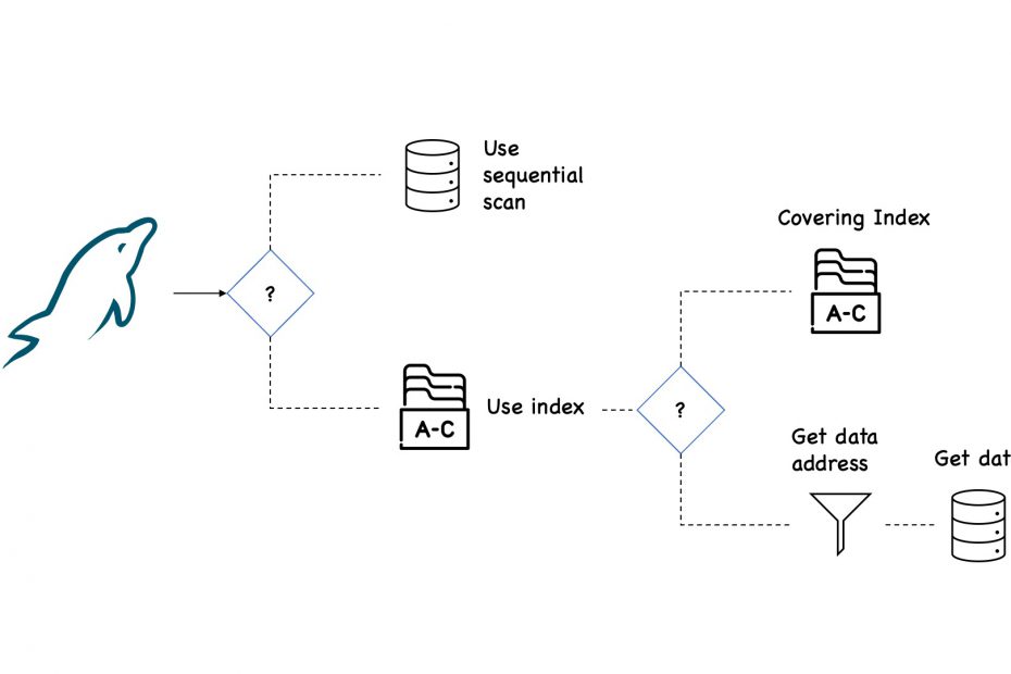
The optimizer has to make a few decisions before executing each query. For example, what is cheaper from a response time perspective?
- Fetch the data directly from a table, or
- Go to an index, and
- Stop here, because all the columns required by client are there in the index, or
- Get the location of the records from the index, and go to the table to get the actual data.
The first method, fetching data directly from the table, is called Full Scan. This is normally the most expensive because all rows must be fetched from the table and checked against a condition. Yet, this method works best for small tables.
In the second set of options, we access an index. If the index has all the necessary data and there is no need to access the table, we have what’s called an Index Only Scan.
But that’s less often the case, so the index is used to filter out rows, and then accessing the table. Usually, this is the cheapest way to access a table. Still, if the client selects a large number of rows, this might not be valid anymore.
Therefore, the optimizer has to make a lot of decisions, based on particular database statistics, before the query is executed. Our goal will then be to observe what the optimizer thinks is the most expensive part of the query so that we could eliminate or enhance that part.
EXPLAIN basics
If you have a slow query, the first thing to try is running it with EXPLAIN. This will show the query plan, in other words, the list of things expected to happen when that query is executed.
If you instead use EXPLAIN ANALYZE before the statement, you’ll get both the estimation of what the planner expected, along with what actually happened when the query ran. Consider the following statement:
EXPLAIN DELETE FROM city;The query is not executed, so it is safe to obtain the query plan. To actually execute the query we can use EXPLAIN ANALYZE as we’ll see later.
This is not only going to show you a query plan for deleting those rows, it is actually going to delete them.
Usually, it’s more difficult to compare the timing of operations when doing INSERT, UPDATE, or DELETE using EXPLAIN ANALYZE. This is because the underlying data will change while executing the same queries.
Optionally, adding the FORMAT option to specify whether you want the result returned in a traditional table format, using the JSON format, or in a tree-style format. Keep in mind that each format will show more or less information about the query plan. For instance, the JSON format is the most verbose of all. Let’s see some use-cases.
EXPLAIN Examples
Single Table, Table Scan
As the first example, consider a query on the city table in the world sample database with a condition on the non-indexed column Name. Since there is no index that can be used, it will require a full table scan to evaluate the query.
EXPLAIN
        SELECT *
          FROM world.city
         WHERE Name = 'London'\G;
*************************** 1. row ***************************
           id: 1
  select_type: SIMPLE
        table: city
   partitions: NULL
         type: ALL
possible_keys: NULL
          key: NULL
      key_len: NULL
          ref: NULL
         rows: 4046
     filtered: 10.00
        Extra: Using where
1 row in set, 1 warning (0.01 sec)
The table access types show whether a query accesses the table using an index, scan, and similar. Since the cost associated with each access type varies greatly, it is also one of the important values to look for in the EXPLAIN output to determine which parts of the query to work on to improve the performance.
The output has the access type set to ALL which is the most basic access type, because it scans all rows for the table. Since this is normally the most expensive access type, the type is written in all uppercase.
It is estimated that 4046 rows will be examined, and for each row a WHERE clause will be applied. It is expected that 10% of the rows examined will match the WHERE clause.
Here, the optimizer uses default values to estimate the filtering effect of various conditions, so you cannot use the filtering value directly to estimate whether an index is useful.
This is the traditional format, however, it doesn’t show the relationship between the subtask so it’s more difficult to have an overview of the query plan.
Formats
Which format is the preferred depends on your needs. For example, the traditional format is easier to use in order to see the indexes used, and other basic information about the query plan, while the JSON format provides much more details.
The tree format is the newest format and supported in MySQL 8.0.16 and later, and is the format we’re going to use for the next examples.
*************************** 1. row ***************************
EXPLAIN: -> Filter: (world.city.`Name` = 'London')  (cost=410.85 rows=405)
    -> Table scan on city  (cost=410.85 rows=4046)
The tree format focuses on describing how the query is executed in terms of the relationship between the parts of the query and the order the parts are executed.
In this case, EXPLAIN output is organized into a series of nodes. At the lowest level, there are nodes that scan tables or search indexes. Higher-level nodes take the results from the lower level ones and operate on them. It can be easier to understand the execution by reading the output from the inside and out.
If you prefer a visual representation of the query plan, Visual Explain from MySQL Workbench is a great option, however, it can’t be used in all situations.
EXPLAIN ANALYZE
The tree format is also the default format for EXPLAIN ANALYZE statement, which is new as of MySQL 8.0.18.
The key difference is that EXPLAIN ANALYZE actually executes the query and, while executing it, statistics for the execution are collected (actual time). While the statement is executed, the output from the query is suppressed so only the query plan and statistics are returned.
EXPLAIN ANALYZE
        SELECT *
          FROM world.city
         WHERE Name = 'London'\G
*************************** 1. row ***************************
EXPLAIN: -> Filter: (world.city.`Name` = 'London')  (cost=410.85 rows=405) (actual time=1.884..4.851 rows=2 loops=1)
    -> Table scan on city  (cost=410.85 rows=4046) (actual time=1.612..4.328 rows=4079 loops=1)
The output gives a good overview of how the query is executed. As mentioned, it can be easier to understand the execution by reading the output from the inside.
First, there is a table scan on city table and then applying a filter for the name.
Here the estimated cost was 410.85 for an expected 4046 rows (per loop). The actual statistics show that the first row was read after 1.612 millisecond and all rows were read after 4.328 millisecond.
There was a single loops, because there was no join to iterate through. In this case, the estimate was not pretty accurate.
Then, these rows are passed to the second phase for filtering, where we see a slight increase in the actual time of execution.
Single Table, Index Access
The second example is similar to the first except the filter condition is changed to use the CountryCode column which has a secondary nonunique index. This should make it cheaper to access matching rows. For this example, all French cities will be retrieved:
EXPLAIN ANALYZE
        SELECT *
          FROM world.city
         WHERE CountryCode = 'FRA'\G;
*************************** 1. row ***************************
EXPLAIN: -> Index lookup on city using CountryCode (CountryCode='FRA'), with index condition: (world.city.CountryCode = 'FRA')  (cost=14.00 rows=40) (actual time=0.133..0.146 rows=40 loops=1)
This time, only a lookup on CountryCode index can be used for the query. The non-unique CountryCode index is used for the table access.
It is estimated that 40 rows will be accessed, which is exactly as InnoDB responds when asked how many rows will match. This is because an index will also bring some statistics with it.
Please observe that, despite returning many more rows than the first example, the cost is only estimated as 0.146 or less than one-tenth of the cost of a full table scan.
Multicolumn Index
The countrylanguage table has a primary key that includes the CountryCode and Language columns. Imagine you want to find all languages spoken in a single country; in that case you need to filter on CountryCode but not on Language.
A query that can be used to find all languages spoken in China is:
EXPLAIN ANALYZE
        SELECT *
          FROM world.countrylanguage
         WHERE CountryCode = 'CHN'\G;
*************************** 1. row ***************************
EXPLAIN: -> Filter: (countrylanguage.CountryCode = 'CHN')  (cost=2.06 rows=12) (actual time=0.042..0.049 rows=12 loops=1)
    -> Index lookup on countrylanguage using PRIMARY (CountryCode='CHN')  (cost=2.06 rows=12) (actual time=0.040..0.045 rows=12 loops=1)
The index can still be used to perform the filtering. The EXPLAIN output shows that the index of Primary Key is used here, but only the CountryCode column of the index is used.
As always, the used part of the index is the leftmost part.
Two Tables With Subquery And Sorting
This query uses a mix of various features and with multiple query blocks.
EXPLAIN ANALYZE
       SELECT ci.ID, ci.Name, ci.District,
              co.Name AS Country, ci.Population
         FROM world.city ci
              INNER JOIN
                (SELECT Code, Name
                   FROM world.country
                  WHERE Continent = 'Europe'
                  ORDER BY SurfaceArea
                  LIMIT 10
                ) co ON co.Code = ci.CountryCode
        ORDER BY ci.Population DESC
        LIMIT 5\\G;
*************************** 1. row ***************************
EXPLAIN: -> Limit: 5 row(s)  (actual time=1.075..1.076 rows=5 loops=1)
    -> Sort: world.ci.Population DESC, limit input to 5 row(s) per chunk  (actual time=1.075..1.075 rows=5 loops=1)
        -> Stream results  (cost=86.69 rows=174) (actual time=0.966..1.061 rows=15 loops=1)
            -> Nested loop inner join  (cost=86.69 rows=174) (actual time=0.965..1.057 rows=15 loops=1)
                -> Table scan on co  (cost=3.62 rows=10) (actual time=0.001..0.002 rows=10 loops=1)
                    -> Materialize  (cost=25.65 rows=10) (actual time=0.946..0.949 rows=10 loops=1)
                        -> Limit: 10 row(s)  (cost=25.65 rows=10) (actual time=0.223..0.225 rows=10 loops=1)
                            -> Sort: world.country.SurfaceArea, limit input to 10 row(s) per chunk  (cost=25.65 rows=239) (actual time=0.222..0.224 rows=10 loops=1)
                                -> Filter: (world.country.Continent = 'Europe')  (cost=25.65 rows=239) (actual time=0.088..0.195 rows=46 loops=1)
                                    -> Table scan on country  (cost=25.65 rows=239) (actual time=0.083..0.161 rows=239 loops=1)
                -> Index lookup on ci using CountryCode (CountryCode=co.`Code`)  (cost=4.53 rows=17) (actual time=0.010..0.010 rows=2 loops=10)
The query plan starts out with the subquery that uses the country table to find the ten smallest countries by area.
Here we can see how the co table is a materialized subquery created by first doing a table scan on the country table, then applying a filter for the continent, then sorting based on the surface area, and then limiting the result to ten rows.
Once the derived table has been constructed, it is used as the first table for the join with the ci (city) table.
The second part of the nested loop is simpler as it just consists of an index lookup on the ci table (the city table) using the CountryCode index:
Here the estimated cost was 4.69 for an expected 18 rows (per loop). The actual statistics show that the first row was read after 0.012 millisecond and all rows were read after 0.013 millisecond. There were ten loops (one for each of the ten countries), each fetching an average of two rows for a total of 20 rows. So, in this case, the estimate was not very accurate (because the query exclusively picks small countries).
-> Index lookup on ci using CountryCode (CountryCode=co.`Code`) (cost=4.69 rows=18)
It is estimated that the join will return 180 rows which comes from the ten rows in the derived table multiplied with the estimate of 18 rows per index lookup in the ci table.
When the nested loop has been resolved using an inner join, the result is streamed (i.e., not materialized) to the sorting, and the first five rows are returned.
Finally, the result is sorted using an internal temporary table and a file sort. The total cost of the query is estimated to be 1.085 milliseconds.
Spotting jumps in runtime
So what can you do with this information? When looking at a plan, there are two questions that you might want to ask yourself:
- Is the runtime shown by the EXPLAIN ANALYZE clause justified for the given query?
- If the query is slow, where does the runtime jump?
Looking for jumps in the execution time of the query will reveal what is really going on. Some general advice is not possible here because there are too many things that can cause issues, but here are some hints.
Inspecting estimates
What we should pay attention to is whether the estimates and actual costs differ from each other. If there is a big difference, the optimizer will make poor decisions. Possible causes for this difference could be that either the optimizer does not have the up-to-date statistics or the optimizer’s estimates are off for some other reason.
Running an ANALYZE TABLE clause is therefore definitely a good thing to start with. However, under normal circumstances, you don’t need to analyse the table, as this happens automatically when certain thresholds are reached.
The index cares for himself, but on high traffic tables, with lots of deletes the index gets “confused” and needs more time to select the right rows, then you run ANALYSE TABLE when no other traffic is made.
So it is definitely worth considering other options that are causing bad estimates. Let’s see such an example.
First, we create a simple table with an autoincrement primary key and an int value. Then, we add an index on the “va”l column.
CREATE TABLE test_estimates (
    id INT AUTO_INCREMENT PRIMARY KEY, val INT);
ALTER TABLE test_estimates ADD INDEX idx(val);
Then, we’ll load some data using python in the mysqlsh tool. The val is also an autoincremented value from 1 to 100k.
queries = [
    ("INSERT INTO `test_estimates`(`val`) values (?)",)
]
for x in range(0, 100000):
    for query in queries:
        sql = query[0]
        result = session.run_sql(sql, (x,))
After loading, we make sure that optimizer statistics are created:
ANALYZE TABLE test_estimates;Let’s have a look at the estimates:
EXPLAIN ANALYZE SELECT * FROM test_estimates WHERE 2 * val < 3\G;

*************************** 1. row ***************************
EXPLAIN: -> Filter: ((2 * test_estimates.val) < 3)  (cost=10102.65 rows=100464) (actual time=0.041..27.369 rows=2 loops=1)
    -> Table scan on test_estimates  (cost=10102.65 rows=100464) (actual time=0.035..19.763 rows=100000 loops=1)
In many cases, MySQL might not be able to estimate the WHERE clause properly, even though it has an index, because it only has statistics on columns, not on expressions. What we can see here is a major overestimation of the data returned from the WHERE clause.
Creating an index on the expression will make MySQL track statistics of the expression.
ALTER TABLE test_estimates ADD INDEX idx_fun((2 * val));

EXPLAIN ANALYZE SELECT * FROM test_estimates WHERE 2*val < 3\G;
*************************** 1. row ***************************
EXPLAIN: -> Filter: ((2 * val) < 3)  (cost=1.16 rows=2) (actual time=0.037..0.040 rows=2 loops=1)
    -> Index range scan on test_estimates using idx_fun  (cost=1.16 rows=2) (actual time=0.036..0.038 rows=2 loops=1)
In this case, trying to avoid the expression on database level is the best choice . However, if that is not possible, adding an index will fix statistics and will also ensure significantly better performance.
The key takeaway from this example is to look at the row counters for estimates vs actual execution. A large difference (i.e., a couple of orders of magnitude or more) between the estimated number of rows and the actual number of rows is a sign that you should look closer at it. The optimizer chooses its plan based on the estimate, but looking at the actual execution may tell you that another plan would have been better.
Hot and cold cache behavior
If you run a query twice, the second will likely be much faster simply because of caching, regardless of whether the plan was better or worse.
This represents “hot” cache behavior, meaning that the data needed for the query was already in the database or operating system caches. It was left in cache from when the data was loaded in the first place. Whether your cache is hot or cold is a thing to be very careful of.
One way to solve this problem is to repeatedly run the query and check if it takes the same amount of time each run. This means that the amount of cached data is staying constant and not impacting results. In this case, it’s 100% cached.
Another way to solve the problem is to clear all these caches out, to get cold cache performance again. However, just stopping the database server isn’t enough, because the operating system cache can be expected to have plenty of information cached. On Linux, you can use the drop_caches feature to discard everything it has in its page cache.
Conclusion
EXPLAIN ANALYZE is a profiling tool for your queries that will show you where MySQL spends time on your query and why. It will plan the query, instrument it and execute it while counting rows and measuring time spent at various points in the execution plan.
It’s important to understand how the queries are actually executed, based on the statistics available.
Once you see how to read query plans and understand how each of the underlying node types work on MySQL, then you should be confident to manage the queries on a production database.
Bibliography
- MySQL 8 Query Performance Tuning, Jesper Wisborg Krogh, Apress, March 2020
- High Performance MySQL, 3rd Edition, Baron Schwartz, Peter Zaitsev, Vadim Tkachenko, O’Reilly Media, Inc., March 2012