Key takeaways:
- Indexes should reduce the amount of read data blocks necessary to answer a query
- Execution plan of a query depends on the data inside the table. If the data has low carnality, PostgreSQL will most probably ignore the index
- When selecting a big portion of the table, PostgreSQL will flip index scans into sequential
Making Use of Indexes
The importance of this topic cannot be stressed enough. Bad indexing is the main source of bad performance. Of course, it is important to adjust memory and vacuum parameters and so on. However, it is all in vain if indexes are not used properly. There is simply no replacement for a missing index. To achieve good performance you need proper indexing.
Understanding simple queries and the cost model
To get started with indexes and understand how things work, some test data is needed. We’ll create a table with 5 million rows using the generate_series function as follow.
pgbench=# CREATE TABLE test_indexing (id serial, name text);
CREATE TABLE


pgbench=# INSERT INTO test_indexing (name) SELECT 'bob'
   FROM generate_series(1, 2500000);
INSERT 0 2500000


pgbench=# INSERT INTO test_indexing (name) SELECT 'alice'
   FROM generate_series(1, 2500000);
INSERT 0 2000000
These 5 million rows have some nice properties. IDs are in ascending order and there are only two distinct values for the name column. If we do a select filtered by id, we’ll a huge response time:
pgbench=# \timing
SELECT * FROM test_indexing WHERE id = 2;

id | name
----+------
  2 | bob
(1 row)

Time: 369.991 ms
Finding the bottlenecks
Let’s see why we got such bad performance. To find out what might be the cause, we’ll use the EXPLAIN command. When a query is not performing well, EXPLAIN will help you understand the real performance problem. Here is how it works:
pgbench=# EXPLAIN SELECT * FROM test_indexing WHERE id = 2;
                                   QUERY PLAN
---------------------------------------------------------------------------
Gather  (cost=1000.00..51617.77 rows=1 width=9)
   Workers Planned: 2
   ->  Parallel Seq Scan on test_indexing  (cost=0.00..50617.67 rows=1 width=9)
         Filter: (id = 2)
(4 rows)
The reason for EXPLAIN is to see what the planner has decided to do in order to run the query efficiently. In this example, PostgreSQL will use a parallel sequential scan. This means that two workers will act together on the filter condition. The partial results are then merged together through a thing called a gather node, which has been introduced in PostgreSQL 9.6. If you look at the details of the query plan, you will see how many rows PostgreSQL expects at each stage of the plan. In this example, one row will be returned since rows = 1.
Deploying simple indexes
Scaling up the number of workers to scan large tables is not the best answer to our performance issue. Scanning the entire table to find a single row is usually not a good idea. Therefore, it makes sense to create indexes:
pgbench=# CREATE INDEX idx_id ON test_indexing (id);
CREATE INDEX
Time: 6739.994 ms (00:06.740)


pgbench=# SELECT * FROM test_indexing WHERE id = 2;
id | name
----+------
  2 | bob
(1 row)
Time: 1.933 ms
PostgreSQL uses Lehman-Yao’s high concurrency btree for standard indexes. Along with excellent performance, these indexes allow concurrent operations. We can read and write on the same index at the same time, which helps to improve throughput dramatically.
However, indexes are not free:
pgbench=# \di+
                                      List of relations
Schema |  Name  | Type  |  Owner   | Table|  Size  | Description
--------+-------+-------+----------+---------+--------+-------------
public | idx_id  | index | postgres | test_indexing    | 107 MB |


pgbench=# \dt+
                          List of relations
Schema |       Name       | Type  |  Owner   |  Size   | Description
--------+------------------+-------+----------+---------+-------------
public | test_indexing    | table | postgres | 192 MB  |
As you can see, our index containing 5 million rows will occupy 107 MB of disk space. Furthermore, writes to the table will be slower because the index has to be in sync all the time.
In this case, the index is certainly not tiny compared to the table. This is the case surprisingly often. Here, it’s more than half the size of the table. You should always take note of how large any index created is relative to the table when determining if it’s a worthwhile addition. The disk and maintenance overhead of an index can be considerable, and it needs to be justified by performance improvement.
In addition, if you insert into a table having many indexes, you also have to keep in mind that you have to write to all those indexes on INSERT, which seriously slows down the writing.
What strategies for indexes are there, and how do they work?
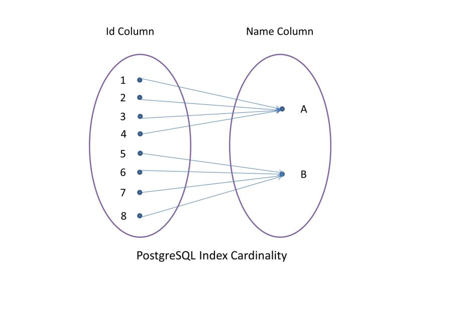
Cardinality – using indexes in an intelligent way
Cardinality is an indicator that refers to the uniqueness of all values in a column. Low cardinality means a lot of duplicate values in that column. For example, a column that stores the gender values has low cardinality. In contrast, high cardinality means that there are many distinct values. For example, the primary key column. When we make a query on a low cardinality column, it’s likely we will receive a large portion of the table. A sequential scan of the table might be more efficient in such cases in comparison to index scans as we will see next.
Until now, for our example, we have used a data structure with only two distinct names but unique IDs. Next, we will want to query the name column, and thus we’ll create an index on that column.
pgbench=# CREATE INDEX idx_name ON test_indexing (name);
CREATE INDEX
Now, it is time to see if the index is used correctly:
pgbench=# EXPLAIN SELECT * FROM test_indexing WHERE name = 'alice';
                              QUERY PLAN
-----------------------------------------------------------------------
Seq Scan on test_indexing  (cost=0.00..87076.00 rows=2507333 width=9)
   Filter: (name = 'alice'::text)
(2 rows)
In this case, PostgreSQL will go for a sequential scan. Question is why is the system ignoring all indexes? The reason is simple: alice and bob make up the entire dataset. PostgreSQL knows this by checking the system statistics. Therefore, PostgreSQL figures he will have to read the entire table anyway. As a result, there is no reason to read both the index and the full table. Simply reading the table is sufficient.
In other words, PostgreSQL will not use an index just because there is one. PostgreSQL will use indexes when they make sense. However, if the number of rows is small, PostgreSQL will consider bitmap scans and index scans.
pgbench=# EXPLAIN SELECT * FROM test_indexing WHERE name = 'alice1';
                                  QUERY PLAN
---------------------------------------------------------------------------
Index Scan using idx_name on test_indexing  (cost=0.43..7.45 rows=1 width=9)
   Index Cond: (name = 'alice1'::text)
(2 rows)
Please observe that alice1 does not exist in the table and the query plan perfectly anticipated this. The metric rows=1 indicates that the planner only expects a 1 row being returned by the query. There is no row in the table which has the name equals to alice1, but PostgreSQL will never estimate zero rows because it would make subsequent estimations a lot harder.
The most important point to learn here is that execution plans depend on input values.
Consequently, execution plans depend on the data inside the table. This is a very important insight, which should be remembered all the time. If the underlying data distribution changes dramatically, execution plans will change as well and this can be the reason for unpredictable runtimes.
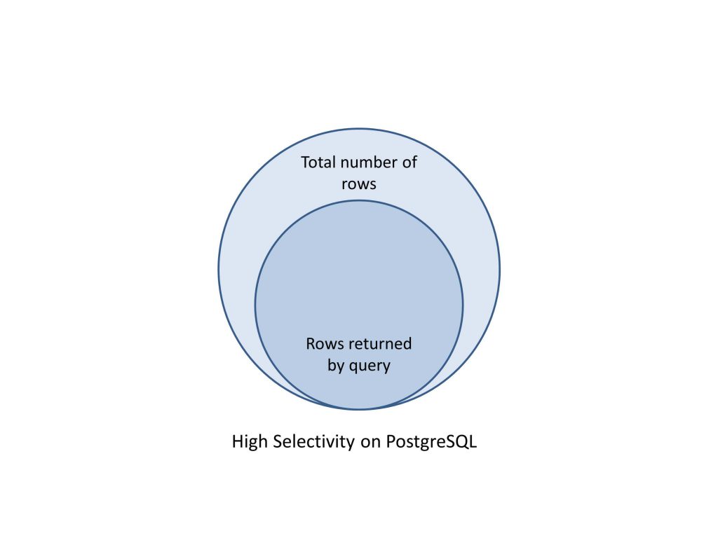
Selectivity – avoid lookups with an inefficient index
Selectivity is a measure of the percentage of rows that will be retrieved by a query. This is usually influenced by the operators used in the filter clauses in the query.
Let’s create another example with a better data distribution. Each key will be an incrementing number, while the values vary from 0 to 10. It’s simple to use generate_series to create data like that:
pgbench=# CREATE TABLE test_indexing2 (id serial PRIMARY KEY,value integer);

pgbench=# INSERT INTO test_indexing2(value)
    SELECT trunc(random() * 10)
        FROM generate_series(1,100000);
Let’s create an index on the value column:
pgbench=# CREATE INDEX idx_value ON test_indexing2 (value);Is this new index worth being created? Consider a simple query that uses it to filter out based on the value:
pgbench=# EXPLAIN ANALYZE SELECT count(*) FROM test_indexing2 WHERE value=1;
                                             QUERY PLAN
--------------------------------------------------------------------------
Aggregate  (cost=780.22..780.23 rows=1 width=8) (actual time=3.635..3.635 rows=1 loops=1)
   ->  Bitmap Heap Scan on test_indexing2  (cost=188.92..755.50 rows=9887 width=0) (actual time=0.912..3.138 rows=9906 loops=1)
         Recheck Cond: (value = 1)
         Heap Blocks: exact=443
         ->  Bitmap Index Scan on idx_value  (cost=0.00..186.44 rows=9887 width=0) (actual time=0.689..0.689 rows=9906 loops=1)
               Index Cond: (value = 1)
Planning Time: 1.411 ms
Execution Time: 3.699 ms
(8 rows)
We expect 1/10 of the table, or around 10,000 rows, to be returned by query. There’s likely to be a value where value=1 on every data block.
Remember that PostgreSQL stores data in blocks of 8Kb. If we wanted to see how many blocks do 100,000 rows occupy we can run the following query and we would get 443 blocks. Also, if we would do the math, we would get around 226 rows per block.
pgbench=# SELECT relname,relpages,reltuples FROM pg_class WHERE relname= 'test_indexing2';

    relname     | relpages | reltuples
----------------+----------+-----------
test_indexing2 |      443 |    100000
(1 row)
Consequently, the system will effectively do two scans of the whole table (443 blocks + 443 blocks=886 blocks), plus the overhead of the index lookup itself. This is clearly a step back from just looking at the whole table.
This behavior, that index scans will flip into sequential ones when they access too much of a table is still surprising to a lot of people.
This whole area is one of the things to be aware of when executing your own queries that are expected to use indexes. You can test them out using some subset of your data. If you then deploy onto a system with more rows or the production system, these plans will change. What was once an indexed query might turn into a full sequential scan.
What can be frustrating for developers is a query coded against a trivial subset of data might always use a sequential scan, just because the table is small and the selectivity of the index is too low. However when the same query is run against the production data set, where the data set is larger, and it will run using an index instead.
Combining indexes – Using bitmap scans effectively
Nevertheless, this doesn’t mean the index on the value column is useless.
This is a common use case when weak criteria can be used together. Let’s suppose we are running something that is selective based on the id column combined with a selection on the value column. Now, maybe 10% of all values are 5, and maybe 10% of all ids are above 9000. Scanning a table sequentially is expensive, and so PostgreSQL might decide to choose two indexes because the final result might consist of just 1% of the data. Scanning both indexes might be cheaper than reading all of the data.
pgbench=# CREATE INDEX idx_id2 ON test_indexing2 (id);

pgbench=# EXPLAIN ANALYZE SELECT count(*) FROM test_indexing2 WHERE id>9000 AND value=5;
In PostgreSQL 10.0, parallel bitmap heap scans are supported. Usually, bitmap scans are used by expensive queries. Therefore, adding parallelism in this area might be a huge step forward and definitely beneficial.
Index bloat
PostgreSQL’s default index type is the binary tree (B-tree). While a B-tree gives good index performance under most insertion orders, there are some deletion patterns that can cause large chunks of the index to be filled with empty entries. Indexes in that state are referred to as bloated. Scanning a bloated index takes significantly more memory, disk space, and potentially disk I/O than one that only includes live entries.
Causes
There are two main sources for index bloat. The first involves deletion. Index pages that have become completely empty are reclaimed for re-use. However, there is still a possibility if all but a few index keys on a page have been deleted. In this case, the page remains allocated.
A second source is that any long-running transaction can cause table bloat and index bloat just because it blocks the efforts of any vacuum procedure to properly clean up tables.
Measuring index bloat
Suppose you create a new table with an index on it. When you insert data into it, the size of the index will grow almost linearly with the size of the table. However, when you have a bloated indexes, the proportion will be different. It’s not unusual for a bloated index to be larger than the actual data in the table. Therefore, you can check if you have a bloated index by watching the index size relative to the table size. This can be checked easily with the following query:
pgbench=# SELECT nspname,relname,round(100 * pg_relation_size(indexrelid) /
        pg_relation_size(indrelid)) / 100 AS index_ratio,
        pg_size_pretty(pg_relation_size(indexrelid)) AS index_size,
        pg_size_pretty(pg_relation_size(indrelid)) AS table_size
      FROM pg_index I
        LEFT JOIN pg_class C ON (C.oid = I.indexrelid)
        LEFT JOIN pg_namespace N ON (N.oid = C.relnamespace)
       WHERE
        nspname NOT IN ('pg_catalog', 'information_schema', 'pg_toast') AND
        C.relkind='i' AND pg_relation_size(indrelid) > 0;

nspname |        relname        | index_ratio | index_size | table_size
---------+-----------------------+-------------+------------+------------
public  | pgbench_branches_pkey |           2 | 16 kB      | 8192 bytes
public  | pgbench_tellers_pkey  |        1.33 | 32 kB      | 24 kB
public  | pgbench_accounts_pkey |        0.16 | 107 MB     | 640 MB
As an example of what this looks like when run, if you create a pgbench database with a scale of 25, the index will be 13% of the size of the table.
Now the index is 2% of the size of the table which looks pretty normal. The exact ratio where we can say that an index is bloated varies depending on the structure of the table and its index. However, if you take a periodic snapshot of this data it’s possible to see if index bloat is growing or not.
Conclusion
In this section, we learned that is important to measure actual block reads to determine whether an index is truly effective. We saw that the execution plans depend on the properties of the underlying data. Even more, it’s noteworthy to know that the execution plan might change based on the volume of data. The same query will execute differently on dev and prod environments.