Key takeaways
- Adding an index increases overhead every time you add or change rows in a table. Each index needs to satisfy enough queries to justify how much it costs to maintain.
- Queries cannot be answered using only the data in an index. The underlying data blocks must be consulted as well.
- Indexes can be quite large relative to their underlying table.
- Indexes can require periodic rebuilding to return them to optimum performance, and clustering the underlying data against the index order can also help improve their speed and usability for queries.
Making use of covering indexes
Consider the following example, which selects two columns from a table:
SELECT id, name FROM person WHERE id = 10;Suppose we have an index on id only. In this case, PostgreSQL will look up the index and do an additional lookup in the table to fetch any extra fields. This method is generally known as an index scan. It needs to do two operations in order to compose a row. First checking the index and then the underlying table.
However, starting with version 11, PostgreSQL supports covering indexes. A covering index is an index that contains extra columns that aren’t part of the index key.
Consider the following example. Given that there are a lot of queries for “name” field although the filtering condition is based on “id” field. There are no filters on the name field itself. To make queries faster, it would make sense to create an index on the id field and include the name field in the index to enable index-only scans. To save some space and build the index faster, it’s rational not to make the name field part of the index key since no queries are expected to filter data using the values of “name” column. The INCLUDE keyword is used for this, as follows:
Indexing foreign keys
When we create a foreign key, we have a parent-child relationship between the tables. The child tables will usually have many more records than the parent table. It’s always a good idea to create an index on the foreign key column in the child table.
There are two reasons why this is useful. First, creating an index improves performance when we join the indexed column. Certainly, we will always be joining the parent and child table on this column. Second, an index improves the speed of execution when we make changes to the parent record. For instance, when deleting a record from the parent table. Not having indexes on foreign key columns can make such operations take a lot of time.
Partial indexes
While we usually create indexes for all records, it’s possible to create an index for a subset of records.
An index created on a subset of data will be smaller than one created without a filter. This will result in an improvement in performance when the index has to be scanned.
For a use case, consider a table that acts as a task management handler. Records that represents tasks needed to be done will be flagged ‘N’. Likewise, tasks that are already processed will be marked with a ‘Y’ flag. After a while, the number of records with flag set to ‘N’ will form a tiny subset of the total dataset. Most records will have the flag set to ‘Y’. It’s likely that the process will query records with ‘N’ flag.
Creating an index for these records where the flag is ‘N’ will be better than creating an index for the entire dataset. The SQL to create the table and index will be:
pgbench=# CREATE TABLE task_manager (
    task_id, is_done );

pgbench=# CREATE INDEX idx_n_done ON task_manager(is_done)
    WHERE is_done= 'N';

pgbench=# CREATE INDEX idx_is_done ON task_manager(is_done);

pgbench=# SELECT pg_size_pretty(pg_relation_size('idx_is_done')),
          pg_size_pretty(pg_relat ion_size('idx_n_done'));
pg_size_pretty | pg_size_pretty
----------------+----------------
120 kB | 48 kB
Reducing space consumption
Indexing’s main purpose is to speed up things as much as possible. As with all the good stuff, indexing comes with a trade-off: space consumption. If your table contains 10 million integer values, the index defined on the table will actually contain these 10 million integer values plus additional overhead.
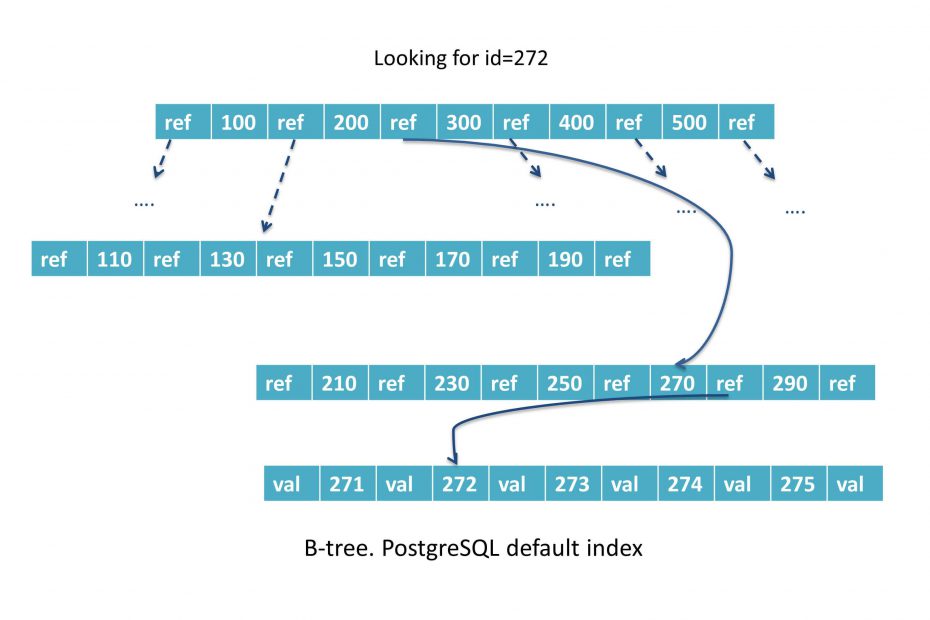
A btree will contain a pointer to each row in the table, and so it is certainly not free to store. We can see how much space an index will occupy, by calling di+ command:
pgbench-# \di+
                                        List of relations
Schema |   Name  | Type  |  Owner   |   Table  |  Size   | Description
--------+-------+-------+----------+------------+---------+----------
public | idx_id     | index | postgres | test_indexing        | 107 MB  |
public | idx_name   | index | postgres | test_indexing        | 107 MB  |
public | idx_random | index | postgres | test_indexing_random | 107 MB  |
In comparison, here is the amount of storage for actual tables.
pgbench-# \d+
                                List of relations
Schema |  Name  |   Type   |  Owner   |    Size    | Description
--------+--------+----------+----------+------------+-------------
public | test_indexing        | table    | postgres | 192 MB     |
public | test_indexing_random | table    | postgres | 192 MB     |
The size of both tables combined is just 384 MB. In comparison, our 3 indexes need more space than the actual data. In the real world, this is common and actually pretty likely. However, is really important to measure the actual use of an index and compare it with its cost. Remember, these indexes don’t just consume space. Every INSERT or UPDATE must maintain the values in the indexes as well. Finally, this vastly decreases write throughput.
If the table has just a few distinct values, partial indexes are a solution:
pgbench=# DROP INDEX idx_name;
DROP INDEX

pgbench=# CREATE INDEX idx_name ON test_indexing (name)
          WHERE name NOT IN ('bob', 'alice');
CREATE INDEX
In this case, the majority of values have been excluded from the index. Therefore, a small, efficient index can be enjoyed:
pgbench-# \di+ idx_name
                                List of relations
Schema |   Name   | Type  |  Owner   |   Table  |    Size    | Description
------+----------+-------+----------+-----------+------------+---------
public | idx_name | index | postgres | test_indexing | 8192 bytes |
(1 row)
It makes sense to exclude very frequent values that make up a large part of the table. It should make up to at least 25% of the total table. Ideal candidates for partial indexes are gender, nationality and so on. However, applying this kind of configurations requires some knowledge of your data, but it definitely pays off.
Improving speed using clustered tables
In this section, you will learn about the power of correlation and the power of clustered tables. This will usually apply when you want to read a whole area of data. For instance, a certain time range.
Two exact same queries executed on two systems might not provide the results within the same time frame, since the physical disk layout might make a difference.
pgbench=# EXPLAIN (analyze true, buffers true, timing true)
   SELECT * FROM  test_indexing WHERE  id < 10000;
                                                          QUERY PLAN
-------------------------------------------------------------------------------------------------------------------------------
Index Scan using idx_id on test_indexing  (cost=0.43..364.84 rows=10766 width=9) (actual time=0.016..3.717 rows=9999 loops=1)
   Index Cond: (id < 10000)
   Buffers: shared hit=4 read=71
Planning Time: 16.935 ms
Execution Time: 4.142 ms
(5 rows)
As you might remember, the data has been filled in sequential way. Data has been added ID after ID, and so it can be expected that the data will be on the disk in a sequential order.
Will things change if the data in your table is in random order?
To create a table containing the same data but in a random order, you can simply use ORDER BY random(). This will ensure that the data is shuffled on disk:
pgbench=# CREATE TABLE test_indexing_random AS SELECT * FROM test_indexing
          ORDER BY random();
SELECT 5000000
Alike our first example, we will add an index column on id columns:
pgbench=# CREATE INDEX idx_random ON test_indexing_random (id);
CREATE INDEX
PostgreSQL will need optimizer statistics in order to operate properly. These statistics will tell PostgreSQL how much data there is, how values are distributed, and whether the data is correlated on disk. To speed things up we will run a manual VACUUM process, which will create statistics about the table. Usually, ANALYZE is automatically executed in the background using the auto-vacuum daemon.
pgbench=# VACUUM ANALYZE test_indexing_random;
VACUUM
Now, let’s run the same query but on the table with random keys.
pgbench=# EXPLAIN (analyze true, buffers true, timing true)
         SELECT * FROM test_indexing_random WHERE id < 10000;
                                                             QUERY PLAN
------------------------------------------------------------------------------------------------------------------------------------
Bitmap Heap Scan on test_indexing_random  (cost=175.63..18208.73 rows=9187 width=8) (actual time=3.162..103.613 rows=9999 loops=1)
   Recheck Cond: (id < 10000)
   Heap Blocks: exact=8252
   Buffers: shared hit=679 read=7603
   ->  Bitmap Index Scan on idx_random  (cost=0.00..173.34 rows=9187 width=0) (actual time=2.016..2.016 rows=9999 loops=1)
         Index Cond: (id < 10000)
         Buffers: shared hit=3 read=27
Planning Time: 0.307 ms
Execution Time: 104.412 ms
(9 rows)
There are a couple of things to observe here. First, an astonishing total of 8500 blocks were needed to satisfy the query and only 679 were served from the cache. The latency has increased dramatically. Certainly, accessing the disk slows things down.
Secondly, you can see that the plan has changed. PostgreSQL now uses a bitmap scan instead of a normal index scan. This is done to reduce the number of blocks needed in the query to prevent even worse performance.
Power of correlation
How does the planner know how data is stored on the disk? pg_stats is a system view containing all the statistics about the content of the columns. The following query reveals the relevant content:
pgbench=# SELECT tablename, attname, correlation
       FROM  pg_stats WHERE tablename IN ('test_indexing','test_indexing_random') ORDER BY 1, 2;

      tablename       | attname | correlation
----------------------+---------+-------------
test_indexing        | id      |           1
test_indexing        | name    |           1
test_indexing_random | id      |  -0.0044142
test_indexing_random | name    |    0.494546
(4 rows)
You can see that PostgreSQL has statistics for every single column. The tables have two columns. In the case of test_indexing.id, the correlation is 1, which means that the next value somewhat depends on the previous one. The same applies to test_indexing.name. First, we have entries containing ‘Bob’ and then we have entries containing ‘Alice’. All identical names are therefore stored together.
In test_indexing_random, the situation is quite different; a negative correlation means that data is shuffled. You can also see that the correlation for the name column is around 0.5. This shows that that names keep switching all the time when the table is read in the physical order.
Why does this lead to so many blocks being hit by the query? The answer is relatively simple. If the data we need is not packed together tightly but spread out over the table evenly, more blocks are needed to extract the same amount of information, which in turn leads to worse performance.
Clustering command
CLUSTER command works by making a whole new copy of the table, sorted by the index you asked for. Once built, the original copy of the data is dropped. CLUSTER process requires an exclusive lock on the table and enough disk space to hold the second reorganized copy. Afterward, you should run ANALYZE to reflect its new ordering in the statistics.
Clustering is a one-time act. Future insertion does not respect the clustered order.
Fill factor
When you create a new index not every entry in every index block is used. A small amount of free space, specified by the fillfactor parameter, is left empty. The idea is that the next set of changes to that index, either updates or insertions, can happen on the same index blocks. Therefore, this will reduce index fragmentation.
The default fillfactor for B-tree indexes is 90%, leaving 10% free space. One situation where you might want to change this is a table with static data. These data won’t change after index creation. In this case, creating the index to be 100% full is more efficient:
CREATE INDEX i ON table(v) WITH (FILLFACTOR=100);However, on tables that are being heavily updated, reducing the fillfactor from its default can reduce index fragmentation, and therefore the amount of random disk access required to use that index.
Combined vs independent indexes
The general rule is that if a single index can answer all your questions, it is usually the best choice. However, you can’t index all possible combinations of fields clients are filtering on.
Let’s suppose we have a table containing three columns: department, last_name, and first_name. An HR application would make use of a combined index like this. You will see that data is ordered by the department column. Within the same department, data will be sorted by last name and first name.
| Query | Possible | Observation |
| department = ‘BI’ AND last_name = ‘Doe’ AND first_name = ‘John’ | Yes | This is the optimal use case for this index. |
| department = ‘BI’ AND last_name = ‘Doe’ | Yes | No restrictions. |
| last_name = ‘Doe’ AND department = ‘BI’ | Yes | No restrictions. |
| department = ‘BI’ | Yes | This is just like an index on ‘department’. However, the combined index obviously needs more space on the disk. |
| first_name = ‘Doe’ | Yes | PostgreSQL cannot use the sorted property of the index anymore. |
Had you instead created three indexes for all columns, those could satisfy each individual type of search, as well as the combined one. You will most likely end up seeing bitmap scans As a result, the response would probably be larger and involve more overhead to update than the multicolumn version. Therefore, it will be a bit less efficient when a query is selecting all columns. a bit less efficient when a query selecting on both columns is run.
Finally, it is a trade-off between efficiency and flexibility.