Key takeaways:
- Queries are executed as a series of nodes that each do a small task, such as fetching data aggregation or sorting.
- Sequential scans give immediate results and are the fastest way to scan small tables or large ones when a significant portion of the table will be returned.
- Index scans involve random disk access and can still have to read the underlying data blocks for visibility checks. But the output is selective and ordered.
- Bitmap index scans use sequential disk reads but allow index selectivity on multiple indexes. There is both time and memory overhead involved in building the hash structure before returning any rows.
- Variation between estimated and actual rows can cause significant planning issues. Looking into the underlying statistics is one way to determine why that’s happening; at a minimum, make sure you have recent statistics from an ANALYZE.
We’ll all have encountered a query that takes just a bit longer to execute than we have patience for. The most effective fix is to perfect the underlying SQL, followed by adding indexes and updating planner statistics. To guide you in these pursuits, PostgreSQL comes with a built-in explainer that tells you how the query planner is going to execute your SQL.
Query execution components
PostgreSQL query execution involves the following four key components:
- Parser: This performs syntax and semantic checking of the SQL string
- Rewriter: This changes the query in some cases; for example, if the query is against a view, the rewriter will modify the query so that it goes against the base tables instead of the view
- Planner: This key component comes up with a plan of execution
- Executor: This executes the plan generated by the planner
Planner Component
The job of the planner is to come up with a series of steps for execution. The plan consists of a tree structure of nodes. Each node could return zero or more tuples. Tuples returned by the child nodes are then used by the parent nodes in the tree until we reach the root node, which returns the results to the client. The planner has to make a few decisions, which we will cover now
Making the decisions
Consider the following query:
SELECT first_name FROM employee WHERE department = 'HR';Now, the optimizer has to make a decision on how to get the data that the user wants. Should it:
- Fetch the data from a table, or
- Go to an index, and
- Stop here because all the columns required are there in the index, or
- Get the location of the records and go to the table to get the data
The first method, fetching data directly from the table, is called Sequential Scan. This works best for small tables.
In the second set of options, we access an index. If the index has all the necessary data and there is no need to access the table, we have an Index Only Scan.
However, if it’s necessary to access the table after accessing the index, there are two options. A bitmapped index scan where a bitmap is created containing the matching tuples. Then, the records are fetched from the table. This is a two-step process, executed one after the other sequentially.
In contrast, the second approach reads the index, and then the table sequentially. These steps will be repeated one after the other many times until matching records are fetched.
EXPLAIN basics
If you have a slow query, the first thing to try is running it with EXPLAIN. This will show the query plan. In other words the list of things expected to happen when that query is executed. If you instead use EXPLAIN ANALYZE before the statement, you’ll get both the estimation of what the planner expected, along with what actually happened when the query ran. Consider the following statement:
EXPLAIN ANALYZE DELETE * FROM table;This is not only going to show you a query plan for deleting those rows, it’s going to delete them. It’s much harder to compare the timing of operations when doing INSERT, UPDATE, or DELETE using EXPLAIN ANALYZE. This is because the underlying data will change while executing the same queries.
Hot and cold cache behavior
If you run a query twice, the second will likely be much faster simply because of caching, regardless of whether the plan was better or worse.
This represents “hot” cache behavior, meaning that the data needed for the query was already in the database or operating system caches. It was left in cache from when the data was loaded in the first place. Whether your cache is hot or cold is a thing to be very careful of.
One way to solve this problem is to repeatedly run the query and check if it takes the same amount of time each run. This means that the amount of cached data is staying constant and not impacting results. In this case, it’s 100% cached.
Another way to solve the problem is to clear all these caches out, to get cold cache performance again. However, just stopping the database server isn’t enough, because the operating system cache can be expected to have plenty of information cached. On Linux, you can use the drop_caches feature to discard everything it has in its page cache.
Query plan node structure
EXPLAIN output is organized into a series of nodes. At the lowest level, there are nodes that scan tables or search indexes. Higher-level nodes take the results from the lower level ones and operate on them. When you run EXPLAIN, each line in the output is a node of the plan. Consider the following example.
pgbench=# explain analyze select * from pgbench_tellers;
                                                  QUERY PLAN
---------------------------------------------------------------------------------------------------------------
Seq Scan on pgbench_tellers  (cost=0.00..8.00 rows=500 width=352) (actual time=0.011..0.037 rows=500 loops=1)
Planning Time: 0.065 ms
Execution Time: 0.057 ms
(3 rows)
This plan has only one node which is a Seq Scan node. The first set of numbers displayed are estimates of the plan, which are the only thing you see if you run EXPLAIN command without ANALYZE clause:
- cost=0.00..8.00. The first cost is the startup cost of the node. That’s how much work is estimated before this node produces its first row of output. In this case, that’s zero, because a Seq Scan immediately returns rows. In contrast, a sort operation is an example of something that takes a while to return a single row. The second estimated cost is for running the entire node until it completes. However, It may not if there is a LIMIT clause on it, in which case it may stop before retrieving all estimated rows.
- rows=500: The number of rows this node expects to output if it runs to completion.
- width=352: Estimated average number of bytes each row output.
The numbers for the actual runtimes show how well this query ran:
- actual time=0.011..34.489: As we can see it took just 37 milliseconds to execute this plan node in total.
- rows=500: As expected, the plan output 500 rows. one of the most common sources of query problems is the difference between the expected rows and the number actually returned by a node.
- loops=1: In our case, there was just one loop. However, nodes such as those doing joins, execute more than once. In that case, the value for loops will be larger than one. As a result, you’ll have to multiply by the number of loops in order to get a total.
Basic cost computation
Query optimizer’s job is to generate possible plans that could be used to execute a query. Then it must pick the plan with the lowest cost to actually execute. The computation cost is done using arbitrary units which are only roughly associated with real-world execution.
- seq_page_cost: How long it takes to read a single page from disk when the expectation is you’ll be reading several that are next to one another. The rest of the cost parameters are relative to this value being the reference cost of 1.0.
- random_page_cost: Read cost when the rows are expected to be distributed randomly across the disk at random. This defaults to 4.0.
- cpu_tuple_cost: How much it costs to process a single row of data. The default is 0.01.
- cpu_index_tuple_cost: Cost to process a single index entry during an index scan. The default is 0.005, lower than what it costs to process a row.
- cpu_operator_cost: Expected cost to process a simple operator or function. If the query needs to add two numbers together, that’s an operator cost. The default is 0.0025.
We can use these numbers to compute the cost shown in the previous example.
pgbench=# SELECT relpages,
         current_setting('seq_page_cost') AS seq_page_cost,
         relpages * current_setting('seq_page_cost')::decimal AS page_cost,
         reltuples,
         current_setting('cpu_tuple_cost') AS cpu_tuple_cost,
         reltuples * current_setting('cpu_tuple_cost')::decimal AS tuple_cost
     FROM pg_class WHERE relname='pgbench_tellers';
relpages | seq_page_cost | page_cost| reltuples| cpu_tuple_cost| tuple_cost
----------+---------------+-----------+-----------+----------------+-------
        3 | 1             |         3 |       500 | 0.01           |      5
(1 row)
You could add the cost to read the pages (3) to the cost to process the rows (5) and you get 8, as shown by the EXPLAIN command in the previous section. This is how you can break down the queries that you are interested in. Eventually, each plan node could be described using the basic five operations. More complicated structures are build based on sequential read, random read, process a row, process an index entry and execute an operator.
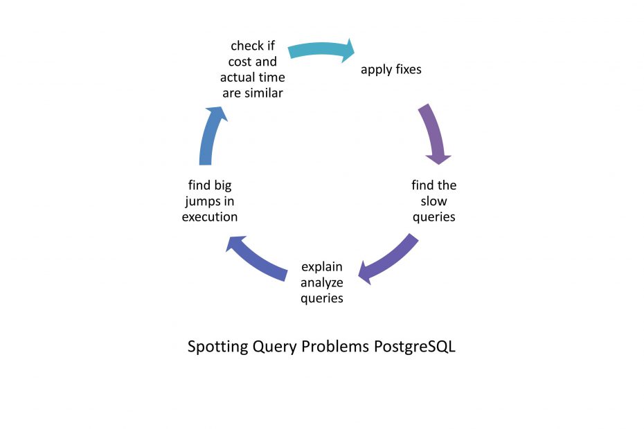
Spotting problems
Spotting jumps in runtime
When looking at a plan, there are two questions that you might want to ask yourself:
- Is the runtime shown by the EXPLAIN ANALYZE clause justified for the given query?
- If the query is slow, where does the runtime jump?
Looking for jumps in the execution time of the query will reveal what is really going on. Some general advice is not possible here because there are too many things that can cause issues.
Inspecting estimates
What we should pay attention to is whether the estimates and actual costs differ from each other. If there is a big difference, the optimizer will make poor decisions. Possible causes for this difference could be that either the optimizer does not have the up-to-date information or the optimizer’s estimates are off for some other reason.
Running an ANALYZE clause is therefore definitely a good thing to start with. However, optimizer stats are mostly taken care of by the auto-vacuum daemon, so it is definitely worth considering other options that are causing bad estimates. Consider the following example.
pgbench=# CREATE TABLE test_estimates AS
            SELECT * FROM generate_series(1, 10000) AS id;
SELECT 10000
After loading, we make sure that optimizer statistics are created:
pgbench=# ANALYZE test_estimates;
ANALYZE
Let’s have a look at the estimates:
pgbench=# EXPLAIN ANALYZE SELECT * FROM test_estimates WHERE sin(id) < 1;
                                                   QUERY PLAN
-----------------------------------------------------------------------------------------------------------------
Seq Scan on test_estimates  (cost=0.00..220.00 rows=3333 width=4) (actual time=0.057..2.198 rows=10000 loops=1)
   Filter: (sin((id)::double precision) < '1'::double precision)
Planning Time: 1.783 ms
Execution Time: 2.546 ms
(4 rows)
In many cases, PostgreSQL might not be able to estimate the WHERE clause properly because it only has statistics on columns, not on expressions. What we can see here is a major underestimation of the data returned from the WHERE clause.
Likewise, it can also happen that the amount of data is overestimated:
pgbench=# EXPLAIN ANALYZE SELECT * FROM test_estimates WHERE sin(id) > 1;
                                                 QUERY PLAN
-------------------------------------------------------------------------------------------------------------
Seq Scan on test_estimates  (cost=0.00..220.00 rows=3333 width=4) (actual time=2.460..2.460 rows=0 loops=1)
   Filter: (sin((id)::double precision) > '1'::double precision)
   Rows Removed by Filter: 10000
Planning Time: 0.112 ms
Execution Time: 2.480 ms
(5 rows)
Fortunately, creating an index will make PostgreSQL track statistics of the expression:
pgbench=# CREATE INDEX idx_sin ON test_estimates (sin(id));
CREATE INDEX

pgbench=# ANALYZE test_estimates;
ANALYZE
In this case, adding an index will fix statistics and will also ensure significantly better performance.
pgbench=# EXPLAIN ANALYZE SELECT * FROM test_estimates WHERE sin(id) > 1;
                                                       QUERY PLAN
------------------------------------------------------------------------------------------------------------------------
Index Scan using idx_sin on test_estimates  (cost=0.29..8.30 rows=1 width=4) (actual time=0.005..0.006 rows=0 loops=1)
   Index Cond: (sin((id)::double precision) > '1'::double precision)
Planning Time: 0.519 ms
Execution Time: 0.050 ms
(4 rows)
Cross-column correlation
Statistics are usually available per column. However, it is also possible to keep track of cross-column statistics, using the CREATE STATISTICS command. This feature has been introduced in PostgreSQL 10. In addition, PostgreSQL can also keep track of statistics for functional indexes. What has not been possible so far is to use more advanced statistics on functional indexes.
Consider the following example of an index covering multiple columns:
CREATE INDEX coord_idx ON measured (a, b, (c * d));
ALTER INDEX coord_idx ALTER COLUMN 3 SET STATISTICS 1000;
Here, we create an index using two simple columns, and we also provide a virtual third column represented by the expression. This new feature allows us to create statistics explicitly for the third column, which would otherwise be suboptimally covered.
In many cases, the fact that PostgreSQL keeps column statistics that do not span more than one column can lead to bad results.
Conclusion
It’s important to understand how the queries are actually executed, based on the statistics available. You should try to adjust the statistics collected and see if anything changes. In addition, try to write new queries and see if the plans you get match what you expected. Certainly, practice is the only way to really become an expert at query optimization. Once you see how to read query plans and understand how each of the underlying node types work on PostgreSQL, then you should be confident to manage the queries on a production database.